Reinforcement Learning – The Big Picture
So, I survived my first week of studying Reinforcement Learning. I know a good amount of deep learning and I love math, so I assumed RL would be an interesting but fairly comfortable excursion. Turns out, it’s much more of a wild frontier – tons of different algorithms, varying and often contradictory advice of what’s best when, and a lot of math.
‘Everything is still exciting — literally nothing is solved yet!’
-Vlad Mnih, Google DeepMind
I dove in first by watching the lecture videos from last year’s Deep RL Bootcamp and working through the accompanying labs. I also read the first three chapters of Sutton and Barto’s Reinforcement Learning textbook. Lastly, I started watching some of the lecture videos from Berkeley’s CS 294 (Fall 2017).
In retrospect, I’d recommend the opposite order – begin with CS 294, then work through the Deep RL Bootcamp labs, and use Sutton & Barto as a reference. I really enjoyed the bootcamp labs – they provide a great framework, but they also don’t feed you every answer, and you do have to understand the various RL algorithms in order to solve them. Lab #2 is specifically about Chainer – if you already know PyTorch, you can probably safely skip this, it’s just a slight change of notation.
The CS 294 lecture videos go much more deeply into the math, but since it’s presented in such a careful and step-wise manner, I found it much easier to follow. Of the bootcamp lectures, definitely check out Nuts and Bolts of Deep RL Research which is full of great practical tips.
For me, most difficult was getting a good overall view of RL. There are so many different algorithms, and often it’s easy to get deep into the math and realize you have no idea why you went there in the first place, and where you are in the bigger picture. I decided to use this blog post to write up a guide to the buzzwords and overall ideas I wish I’d known a week ago.
How is Reinforcement Learning different from Deep Learning?
In deep learning, we train a network by giving it input and then telling it what its output should be. We assign a cost based on how far the network’s answer is from the correct answer, and then train the network to minimize that cost.
In reinforcement learning, we no longer immediately tell our system what the correct answer should be. If our program is playing tic-tac-toe, it has to make several different decisions, and then only at the end it finds out if it won, lost, or tied. The difficulty in RL is how to take that final reward and use it to improve the game strategy. If the program lost, what does it do with this information? Does it blame all its moves, or the most recent moves, or the moves that were different than the game it won? In order to deal with this uncertainty, we need to play many, many games.
S, A, R, and sometimes O
RL deals in States (S), Actions (A), and Rewards (R). State S is all the information about the world now. For a video game, this might be all the screen pixels. For a robot, it might be the camera pixels and all of its own joint angles. Given S, our agent has to choose action A. We tell the environment our choice, and it tells us what our next state is.
Our agent’s goal in life is to maximize expected reward R. It does this by learning to choose “good” actions.
We might live in a deterministic world (like Pacman) where taking action A on state S automatically puts us in a new state S’, but often we’re in a stochastic one, where the outcome is probabilistic.
Observations O come into play if we as the agent don’t know everything about the world state S. We usually accept that O is a good approximation of S, but it’s good to remember these are separate.

Expected reward deals with uncertainty in a stochastic world. If my odds of winning the $10M lottery are 1 in 5 I’ll buy a ticket (a $2M expected reward for my $1 ticket sounds great!). If the odds of winning are 1 in a billion, I’ll probably pass.
Markov Decision Process
This is a fancy name for a simple idea – the way the environment transitions from S(t) to S(t+1) depends only on S(t) and A(t). There’s no looking back in time, and the environment doesn’t care about any of the states and actions in the past.
At first glance, it’s not obvious how this relates to real life at all. If you’re looking at a ball flying through the air, the current position is clearly not enough to tell you what the ball’s next position will be. To make this work, you have to be careful about what information S includes. In the case of our ball, S also needs to include the velocity and even things like the wind speed.
Although a simple idea, MDP is quite powerful. It means we can choose our action only based on our current state. We don’t need to consider all past states and actions. Also, the transition operator – the way the world moves from the current state-action pair [S(t), A(t)] to the next state S(t+1) – is linear.
Policy Gradients
Policy Gradient is a very popular category of RL methods. Here we look to learn a policy, which prescribes what action to take, given the state of the world. We usually want policy π to be continuous: π(A|S) tells us the probability of choosing action A, given state S.

In a few moments, a good policy would tell me to turn my car about 90° to the right. I’m ok with a chance I’ll be anywhere in the range 85-95°. Hopefully there’s a vanishingly small chance I’ll accidentally turn 90° left.
In addition to mirroring real life, a continuous policy means we have a continuous expected reward function. This is hugely important, since we can then take a gradient and use this to improve our policy.
Often we implement the policy as a neural net, with weights θ. In traditional deep learning, we would train this neural net by defining a loss function, and then optimizing the model to minimize this loss. At each step we take the gradient of the loss function with respect to each of our weights (this is backprop), and then we take a step in the direction that minimizes loss.
We’d like to do the same thing here except we no longer have a nice expression to differentiate. We’re now looking to maximize expected reward. Given that we’ll get stochastic rewards over time based on our policy, this is quickly a mess. Rather than try to use backprop to figure this out analytically, we’ll use…
Monte Carlo Sampling
In RL, we’re often faced with integrals that we can’t solve analytically. We can express our expected reward as an integral over all possible trajectories, but we don’t have a good way to express any of this as a specific function we could integrate. Instead, we can sample a lot of trial runs, and use that to figure out our expected reward.

Monte Carlo sampling is used to calculate difficult integrals. In RL, we use it to calculate the expected reward (using the rewards we get from all our different simulation runs).
One trouble — what if our dart-thrower is biased, and more often hits the left-hand side of the board? This is the problem we run into when sampling the Policy Gradient (we’re sampling trajectories according to our policy, not according to all the equally possible random trajectories). We use a very neat trick to rescue this situation, the Log Likelihood trick.
Another big issue – if we change our policy slightly, we then have to redo all our samples. There are a few common buzzwords to describe this – policy gradient is an “on-policy” learning technique, and it is not very “sample efficient”. Maybe we have a fast simulator and don’t care about this time, but maybe we have an expensive and slow robot and would be better off choosing a different technique such as…
The Q-Function
The other main approach to finding a good policy is to first represent the value of each state. We set Value V(S) to be the expected reward we’d get if we start at S and follow our policy until the end of our trial run. Adding a very slight twist, we could instead track a Q-function. This is nearly the same thing, except here we express the expected reward from state S if we now take action A.
For both V and Q, we can look at the values for a particular policy, or we could consider V* and Q* for an ideal policy – the best expected reward we could get from each state. If we knew that ideal Q*, then at each state S we should just choose the action that maximizes it.
The trouble of course is that we don’t know V* or Q* a priori. We generally start with a randomized, nonsense Q, and then look for ways to improve it.
Tabular Q-Learning vs. Deep Q-Networks (DQN)
This depends on the size of our world — can we fit all our states S and actions A in a nice lookup table? If so, we’re in the world of Tabular Q-Learning. If not, we need a formula, or some other way to generate our Q for each S and A. We could look to fit some linear function, or more often we throw a neural net at the problem.
ε-Greedy
There is a constant tension between Exploration (trying out new paths) and Exploitation (sticking to the actions you know will yield good rewards). In Q-Learning, our “best” action is the one that maximizes Q. However, if we only ever take this action, we won’t explore other options, and we might totally miss a different route that is much more rewarding.
We use ε-Greedy to address this. Some small percent of the time (say ε=.1), we take any random action other than our best action. The rest of the time, we choose the greedy option (the one with the highest reward). We could start out with a high ε, and then lower it as our Q-function gets more accurate and we’re more sure that we know which states are good.
Fake it ’til you make it
Turns out, this is not just my own favorite motto, but also the way most of reinforcement learning works.
The goal in RL is to find a way to maximize expected reward. We do this by learning a good policy π (in Policy Gradient methods) or a good Q-Function (in Q learning). Or we could learn some combination of the two (hint: Actor-Critic methods), but I’ll get to that next week.
However, in any of these cases, we usually start things out by initializing all our parameters randomly.
The magic comes in when we evaluate how our policy performed, and use this to figure out how to improve π or Q. As we iterate over and over, we hope that little by little we’re getting better, and eventually we’ll reach our goal.
This raises several interesting questions — how do we know we’re going to get better? Are we guaranteed to converge to some final policy? Will it be a good final policy? How long will it take to converge? Could starting out at a different random initialization yield a wildly different outcome? Are there tricks we could use to reduce variance and make our algorithm more likely to succeed? How do we pick which algorithm to use?
A lot is already known about these topics, but in many cases, these are still open questions.

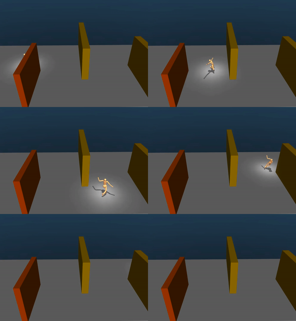
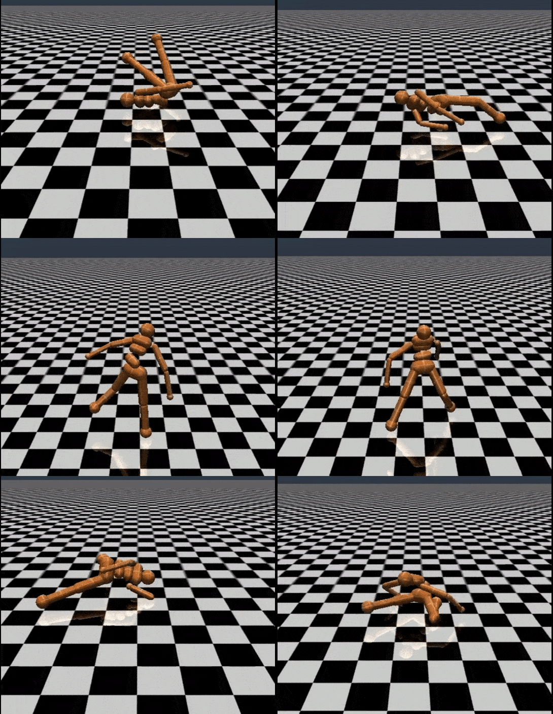
Google DeepMind’s humanoid run. Converging on a policy doesn’t automatically guarantee it’s the best policy…
Upcoming…
Next week I’m planning to continue my exploration of RL. In my blog post I’ll do a quick tour through various RL algorithms and I’ll write a bit about the math behind this all. I’m also planning to watch more Berkeley CS 294 lectures and work through those labs, so I’ll report back on what I learn!


